Statistical analysis in R #

Learning outcomes #

By the end of this topic, you should be able to

summarise data in contingency tables
calculate basic statistics from data
- in particular, calculate dependency measures of two variables
simulate random observations

Warning: the materials here are so-called “Base R”. There are easier (and often better) ways of doing things with the “tidyverse” ecosystem (see next section).

Note that page numbers refer to the book The R Software.

Understanding your data - Importing data - Pages 339-343 #

We will use the sample_data.csv data throughout this module

download the data from Moodle
set-up the working directory and import the data (recommended to save the data in the folder you set as working directory)
use the attach() function to gain direct access to the variables

sample_data <- read.csv("sample_data.csv", header=TRUE)
attach(sample_data)
head(sample_data)
##   X gender situation tea coffee height weight age      meat      fish raw_fruit
## 1 1 Female    single   0      0    151     58  58 4-6/week. 2-3/week.  <1/week.
## 2 2 Female    single   1      1    162     60  60    1/day.   1/week.    1/day.
## 3 3 Female    single   0      4    162     75  75 2-3/week.  <1/week.    1/day.
## 4 4 Female    single   0      0    154     45  45     never 4-6/week. 4-6/week.
## 5 5 Female    single   2      1    154     50  50    1/day. 2-3/week.    1/day.
## 6 6 Female    single   2      0    159     66  66 4-6/week.   1/week.    1/day.
##   cooked_fruit_veg    chocol       fat
## 1        4-6/week.    1/day.     Isio4
## 2           1/day.  <1/week. sunflower
## 3          1/week.    1/day. sunflower
## 4            never 2-3/week. margarine
## 5           1/day. 2-3/week. margarine
## 6           1/day.  <1/week.    peanut

Understanding your data - Variables - Pages 339-343 #

13 variables (columns) of 226 individuals (rows)

qualitative: gender, situation and fat
ordinal: meat, fish, raw_fruit, cooked_fruit_veg and chocol
discrete quantitative: tea, coffee
continuous quantitative: height, weight and age

Notes

The sample_data.csv is created based from the nutrition_elderly.csv spreadsheet downloaded from http://www.biostatisticien.eu/springeR/nutrition_elderly.xls. See Page 339.
Variables of nutrition_elderly.csv have been structured following the steps from Pages 340-343 and a new data frame was created and saved as sample_data.csv.

Frequency tables #

Frequency table - discrete variables - Pages 343-344 #

For qualitative variable fat:

(tc <- table(fat))
## fat
##    butter      duck     Isio4 margarine     olive    peanut repesseed sunflower 
##        15         4        23        27        40        48         1        68
(tf <- tc/length(fat))
## fat
##      butter        duck       Isio4   margarine       olive      peanut 
## 0.066371681 0.017699115 0.101769912 0.119469027 0.176991150 0.212389381 
##   repesseed   sunflower 
## 0.004424779 0.300884956
nlevels(fat)
## [1] 0

A similar table can be obtained using dplyr:

sample_data %>% group_by(fat) %>% summarise(n = n())
## `summarise()` ungrouping output (override with `.groups` argument)
## # A tibble: 8 x 2
##   fat           n
##   <chr>     <int>
## 1 butter       15
## 2 duck          4
## 3 Isio4        23
## 4 margarine    27
## 5 olive        40
## 6 peanut       48
## 7 repesseed     1
## 8 sunflower    68

Frequency table - continuous variables - Page 344 #

For the continuous variable ‘height’, using dplyr functions (and function cut() to create intervals of ‘height’), we get:

sample_data %>% 
  mutate(ints = cut(height, breaks= c(140,150, 160, 170, 180, 190), right = F)) %>%
  group_by(ints) %>%
  summarise(n = n())
## `summarise()` ungrouping output (override with `.groups` argument)
## # A tibble: 5 x 2
##   ints          n
##   <fct>     <int>
## 1 [140,150)     3
## 2 [150,160)    70
## 3 [160,170)    89
## 4 [170,180)    52
## 5 [180,190)    12

A similar table can be obtained in base R (but it’s hard to get appropriate names for categories!):

res <- hist(height, plot=FALSE, breaks = c(140,150,160,170,180,190), right = F) # put the data in 5 categories
x   <- as.table(res$counts) # create the table
nn  <- as.character(res$breaks)
dimnames(x) <- list(paste(nn[-length(nn)], nn[-1],sep="-")) # add names to categories: this step is not straightforward!
x
## 140-150 150-160 160-170 170-180 180-190 
##       3      70      89      52      12

Frequency table - Choice of the interval brackets #

The choice of the interval brackets is arbitrary. There are no specific rules to choose the break points, but the choice should make practical sense. It mainly depends on the dataset, and the objective of the analysis.

sample_data %>% 
  mutate(ints = cut(height, breaks= c(140,145,150,155,160,
    165,170,175,180,185,190), right = F)) %>%
  group_by(ints) %>%
  summarise(n = n())
## `summarise()` ungrouping output (override with `.groups` argument)
## # A tibble: 10 x 2
##    ints          n
##    <fct>     <int>
##  1 [140,145)     1
##  2 [145,150)     2
##  3 [150,155)    33
##  4 [155,160)    37
##  5 [160,165)    54
##  6 [165,170)    35
##  7 [170,175)    31
##  8 [175,180)    21
##  9 [180,185)     6
## 10 [185,190)     6

sample_data %>% 
  mutate(ints = cut(height, breaks= c(140,160,180,200), right = F)) %>%
  group_by(ints) %>%
  summarise(n = n())
## `summarise()` ungrouping output (override with `.groups` argument)
## # A tibble: 3 x 2
##   ints          n
##   <fct>     <int>
## 1 [140,160)    73
## 2 [160,180)   141
## 3 [180,200)    12

Frequency table - joint observations - Pages 344-345 #

For the paired observations of gender and situation:

(mytable <- table(gender,situation))
##         situation
## gender   couple family single
##   Female     56      7     78
##   Male       63      2     20
(table.complete <- addmargins(mytable, FUN=sum, quiet=TRUE))
##         situation
## gender   couple family single sum
##   Female     56      7     78 141
##   Male       63      2     20  85
##   sum       119      9     98 226

Numerical statistics - Pages 347-352 #

Some useful statistics for a preliminary analysis (of variable ‘weight’ in this example):

mean(weight)
## [1] 66.4823
median(weight)
## [1] 66
sd(weight)
## [1] 12.03337
max(weight)-min(weight)
## [1] 58
IQR(weight)
## [1] 17.75
mean(abs(weight-mean(weight)))
## [1] 9.919884
quantile(weight, probs=c(0.1,0.9))
##  10%  90% 
## 51.5 82.0

Numerical statistics - Notes - Pages 347-352 #

We’ve seen some examples of statistical functions, but there exists many more and with what you now know you can create your own functions to perform analysis.
Always make sure you understand the outcome of your codes.
An important problem in real data sets is that of missing data. In R you can check for missing data using the function na.fail(), and remove the missing data with na.omit() (see Page 347).
You should also inspect whether your data is ‘valid’. For example, if there is a human height of 3 meters, then it is most likely an invalid data point.

Discussion - Spot data problems #

Do you see any problems in the data set below?

(my.data <- data.frame(
             StudentID =c("001", "002", "008", "007", "002"), 
             First_Name =c("01iver", "Emily", "Sofia", "Alex", "Emilia"), 
             Last_Name =c("Smith", "Jones", "Williams", "Brown", "Jones"), 
             BirthDate =c("M", "F", "F", "W", "F"), 
             DateOfBirth=as.Date(c("18/01/1998","29/02/1998","11/12/1997","05/07/1998","19/03/1998"),"%d/%m/%Y"),
             DateOfEnrollment=as.Date(c("31/01/2018","02/02/2016","01/07/2016","02/07/2019","05/02/1997"),"%d/%m/%Y"),
             University =c("UNSW",NA,"UNSW","UNSW","UNSW"),
             WAM=c(52,67,76,87,92),
             Grade=c('P','C','D','HD','D'),
             Books_Borrowed=c(15,6,7,2.3,9),
             Lib_Fines_Incurred=c("$20","$0","$0","$24","$0")
            )
           )
##   StudentID First_Name Last_Name BirthDate DateOfBirth DateOfEnrollment
## 1       001     01iver     Smith         M  1998-01-18       2018-01-31
## 2       002      Emily     Jones         F        <NA>       2016-02-02
## 3       008      Sofia  Williams         F  1997-12-11       2016-07-01
## 4       007       Alex     Brown         W  1998-07-05       2019-07-02
## 5       002     Emilia     Jones         F  1998-03-19       1997-02-05
##   University WAM Grade Books_Borrowed Lib_Fines_Incurred
## 1       UNSW  52     P           15.0                $20
## 2       <NA>  67     C            6.0                 $0
## 3       UNSW  76     D            7.0                 $0
## 4       UNSW  87    HD            2.3                $24
## 5       UNSW  92     D            9.0                 $0

Furthermore, what functions can you use to check for these mistakes?

Discussion - Solution #

Oliver spelt with zero and one instead of ‘Ol’
Different names with same StudentId
Gender: value ‘W’ is not consistent
Invalid DateOfBirth: There is no 29th in February in 1998
DateOfEnrollment before DateOfBirth
University: Missing data
Invalid value of Grade: WAM of 92 should correspond to HD rather than D
Books_Borrowed: Decimal numbers
Lib_Fines_Incurred are character variables rather than numeric

To check for mistakes, one can:

Statistical functions: minimum, maximum, frequency table, mean, etc.
str(), typeof() to check format
is.na(my.data)
na.omit(my.data) to remove rows with missing values

Dependency (association) measures - Pages 354-355 #

We introduce the cor() function which allows one to calculate three dependency measures.
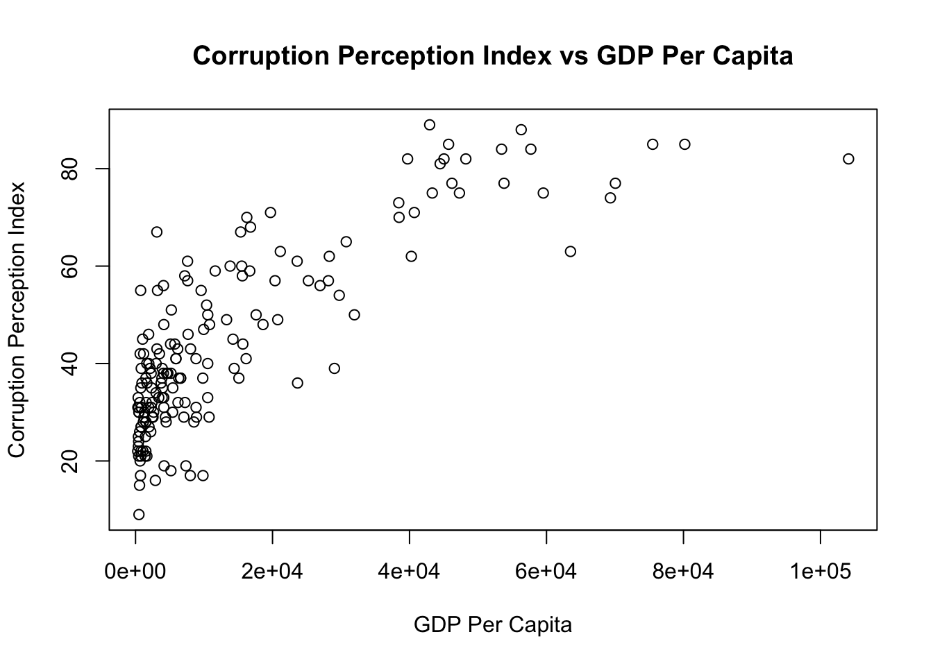
As an example, we compute the correlation between two variables: ‘GDP per Capita’ and ‘Corruption Perception Index’. This index ranks countries by ‘their perceived levels of public sector corruption according to experts and business people’ ( reference). Note that the lower this index, the more corrupt a country is (or is perceived to be).

# Load dataset
cor.example <- read.csv("correlation.csv", header = T)

#Compute association measures
cor(cor.example$GDP.Per.Capita, cor.example$Corruption.Perception.Index, method="pearson")
## [1] 0.8105382
cor(cor.example$GDP.Per.Capita, cor.example$Corruption.Perception.Index, method="kendall")
## [1] 0.5833383
cor(cor.example$GDP.Per.Capita, cor.example$Corruption.Perception.Index, method="spearman")
## [1] 0.7640715

We note a high correlation between GDP per Capita (in US$) and Corruption Perception Index. That being said, from the graph we see that the relationship is not linear but convave.

Notes:

All three measures yield values ranging from -1 to 1.
Pearson’s correlation is probably the most widely used dependency measure. However, one should be aware that it only measures linear association.
Although Kendall’s tau and Spearman’s rho are related to correlation, they measure non-linear dependencies. You will learn the theoretical details of these dependency measures in more advanced courses.
Data for this example comes from: transparency.org and data.worldbank.org.

Case Study: ‘Big Data’ Example #

We introduce here two ‘big’ data sets, which contain insurance data. Those are the files

$\verb|file_policy_building.csv|$, which contain information on all policies sold
$\verb|file_claim_building.csv|$ , which contain information on all claims made, from the policies sold

Additional information on these data sets can be found in the file $\verb|data_note.pdf|$.

Here we want to analyse this data to get insights on it. As a first step, import both data sets in $\verb|R|$, and check what they look like.

Hint: use function $\verb|head()|$.

Case Study: Import and check #

# Import files
building_policy <- read.csv("file_policy_building.csv")
building_claim <- read.csv("file_claim_building.csv")

# Check the first few rows of both files
head(building_policy)
##     PolicyID  Inception     Expiry Age   GeoRisk   SocRisk
## 1 B000000001 2007-10-02 2008-10-01  37  Low Risk  Low Risk
## 2 B000000002 2009-12-25 2010-12-24  48 High Risk  Low Risk
## 3 B000000003 2012-05-28 2013-05-27  46  Low Risk High Risk
## 4 B000000004 2010-03-27 2011-03-26  34  Low Risk High Risk
## 5 B000000005 2015-01-17 2016-01-16  42 High Risk  Low Risk
## 6 B000000006 2014-06-21 2015-06-20  41  Low Risk    Normal
head(building_claim)
##     PolicyID AccidentDay GrossLossBuilding
## 1 B000000018  2008-11-24          454.3947
## 2 B000000020  2009-10-11         2576.5590
## 3 B000000022  2009-10-15         1012.0273
## 4 B000000029  2012-12-07          696.5213
## 5 B000000031  2006-12-09          858.4258
## 6 B000000032  2014-01-15         1636.9965

What do you see? Can you describe the information contained in those data sets?

Case Study: Exploration Questions #

Using $\verb|R|$, try to answer the following questions:

How many different policies are there?
How many claims were made?
How many distinct policies generated claims?
Why are the answers to question $2.$ and $3.$ different?

Exploration Questions: Solution #

# Number of policies in total
length(building_policy$PolicyID)
## [1] 1048577
# Number of claims in total
length(building_claim$PolicyID)
## [1] 310751
# Number of DISTINCT policies with a claim
length(unique(building_claim$PolicyID))
## [1] 262286

We see that there are much more policies than claims; this makes sense as not all insured will make claims.
Also, there are fewer distinct policies making claims than the total number of claims. This also makes sense, as it is possible that the same policy generates more than one claim.

Advanced Questions #

You may have noticed that each policy has a ‘GeoRisk’ category, either ‘Low Risk’, ‘Normal’, or ‘High Risk’. We want to know if these risk categories are appropriate. That is, are there more claims on average for policies categorised as ‘High Risk’? And are those claims bigger than for lower risk categories?

Questions:

For each category of ‘GeoRisk’, find the average number of claims per policy.
For each category of ‘GeoRisk’, find the mean and standard deviation of the total claim amount per policy (so if the same policy generates many claims, we want the total amount)

Hint: you will have to merge the two files. Also, don’t forget your new friend $\verb|dplyr|$!

Advanced Questions: Solution #

# We first merge the files
# The 'all.y = TRUE' is very important, because it will keep the policies with more than one claim
building_all <- merge(x=building_claim, y=building_policy, by = "PolicyID", all.y=TRUE)

# Our solution uses dplyr:
building_all %>%
  # Create a variable 'claim_ind' which is 1 if there is a claim (for a given policy), 0 otherwise
  # Create a variable 'claim_amount' equal to the claim amount (GrossLossBuilding) if there is a claim, 0 otherwise
  mutate(claim_ind = ifelse(is.na(building_all$AccidentDay), 0, 1), 
         claim_amount = ifelse(is.na(building_all$AccidentDay), 0, GrossLossBuilding)) %>%
  # Group all rows that are the same policy, count the number of claims in each, and the total claim amount
  group_by(PolicyID) %>% mutate(num_claim = sum(claim_ind), sum_claim = sum(claim_amount)) %>% 
  # Keep only one row per PolicyID
  distinct(PolicyID, .keep_all = T) %>%
  # Finally, group by GeoRisk and find the statistics
  group_by(GeoRisk) %>% summarise(mean.nb = mean(num_claim), mean.amount = mean(sum_claim), sd.dev = sd(sum_claim))
## `summarise()` ungrouping output (override with `.groups` argument)
## # A tibble: 3 x 4
##   GeoRisk   mean.nb mean.amount sd.dev
##   <chr>       <dbl>       <dbl>  <dbl>
## 1 High Risk   0.429       1186.  2174.
## 2 Low Risk    0.210        116.   294.
## 3 Normal      0.317        438.   918.

Do you think the risk categories are appropriate?

Advanced Questions: Discussion #

The risk categories do seem appropriate, since both the frequency (number of claims) and severity (size of claims) are the highest for the ‘High Risk’ category, and the lowest for the ‘Low Risk’ category.
The standard deviation for the ‘High Risk’ category is also much higher, indicating a lot of variability in the claim size.
Can you think of any other analysis you would want to do with this dataset? Maybe check if there is a link between the ‘Age’ of an insured and their number/size of claims? What else?

Probability distributions and random variables in R #

As seen in the prerequisite course ZZBU6501 (Introductory Data Analysis), statistical analysis is concerned with understanding and modelling random variables. This is important, as random variables are mathematical descriptions of the random phenomena encountered in everyday life
Many probability distributions are implemented in base R. There are typically four functions you can use for each distribution. For the Normal distribution they are dnorm (density function), pnorm (CDF), qnorm (quantile function) and rnorm (random generator)

dnorm(1.96, mean = 0 , sd = 1)
## [1] 0.05844094
pnorm(1.96, mean = 0 , sd = 1)
## [1] 0.9750021
qnorm(0.975, mean = 0 , sd = 1)
## [1] 1.959964
rnorm(1, mean = 0, sd = 1)
## [1] 0.8650636

Many more probability distributions are implemented in R. For instance, can you guess what dexp() does? Or pgamma()?

Generating random variables in R - Page 74 #

To conduct statistical analysis, it is often useful to be able to generate realisations from random variables, and R is an apt tool to do so throught the use of functions runif(), rnorm(), rgamma(), etc…

# Generate two random obervations from a Uniform[0,1]
runif(n = 2)
## [1] 0.8510166 0.7857717
# Generate four random observations from a Uniform[2,7]
runif(n = 4, min=2, max=7)
## [1] 5.480644 5.216459 2.914898 4.077222

Generate random variables in R - set.seed() #

R cannot generate observations that are completely random. The simulated values are generated with an algorithm that ‘imitates’ randomness. It looks random, and is random in the sense that if you don’t know the algorithm (and where it starts), there is no way you can predict the numbers that will come out. But if you do know the algorithm (and where it starts), then you can predict the numbers precisely.
Hence, it is possible to replicate simulated ‘random’ values, provided you start the algorithm at the same place as before.
To do so, use function set.seed(). When setting the seed to any particular value and then generating a random number, you are guaranteed to obtain the same result. Have a look at this example:

# I don't set the seed:
rnorm(1)
## [1] -0.7679273
rnorm(1)
## [1] 0.3614276

# I set the seed
set.seed(7)
rnorm(1)
## [1] 2.287247
set.seed(7)
rnorm(1)
## [1] 2.287247

# I set a different seed
set.seed(3)
rnorm(1)
## [1] -0.9619334
set.seed(3)
rnorm(1)
## [1] -0.9619334

Relevant Exercises #

5.14-5.19, 11.1-11.13