htmlwidgets - visNetwork #
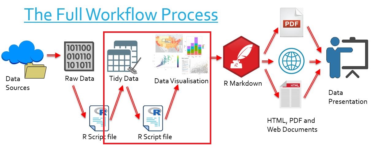
The Bigger Picture #
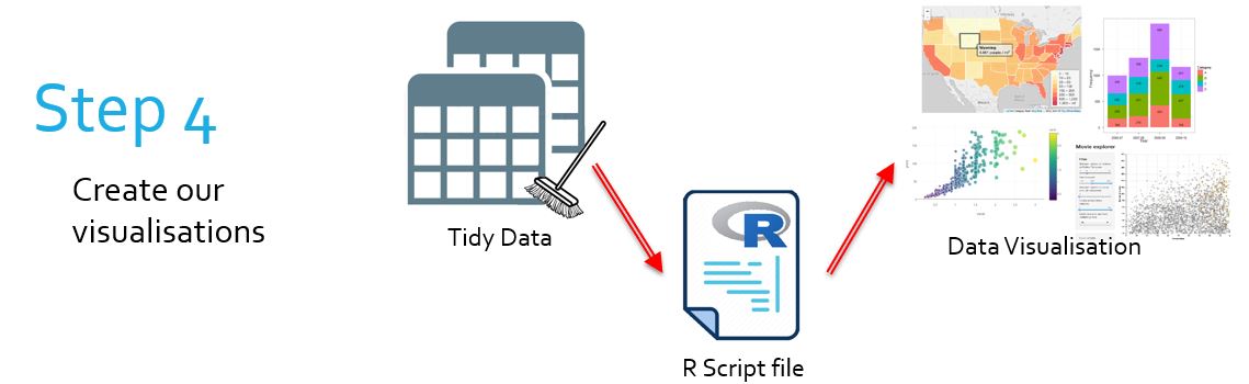
In this document we learn how to create interactive networks with visNetwork. Simply put, we are learning how to transform tidy data into visually clear graphs. In the overall context of the workflow, this falls into the category of transforming our data into data visualisation.
What is visNetwork? #
library("tidyverse")
library("visNetwork")
- An htmlwidget used to make interactive networks from data frames and tibbles
- It is a package which allows for a unique (and fun) interactive visualisation of the connections within data
- Networks can visualise relationships, such as in the following predator-prey example:
- It is essentially the best package for visualising networks
- The package is bound to the vis.js library in JavaScript
Creating Very Basic Networks #
The very first thing we will do is create a network based on some very easy data. The data is easy because everything will be provided for us.
Whenever we create a visNetwork chart, the network requires two data frames (or tibbles)
- One of these contains information about the “nodes” of the data. The nodes are the things we are trying to find a relationship between.
- Eg cities
- One of these contains information about the “edges” of the data. The edges connect the nodes, and represent some relationship between the nodes.
- Eg distance between the cities
We explain how to create these in R using an example: we have 5 people, and we wish to graphically represent which people know which other people. In our example, a person is a node, and an edge represents that two people know each other.
We will use the readxl package to read in our data from two Excel files:
library("readxl")
net_nodes <- read_xlsx("Sample_network/nodes.xlsx")
net_edges <- read_xlsx("Sample_network/edges.xlsx")
Let’s take a look at each dataframe more closely:
net_nodes
## # A tibble: 5 x 2
##      id label
##   <dbl> <chr>
## 1     1 Michael
## 2     2 Sarah
## 3     3 Thomas
## 4     4 Joshua
## 5     5 Rachel
The “nodes” dataframe contains two columns: id and label. id numbers each observation 1-5. label labels each observation with their name.
net_edges
## # A tibble: 7 x 2
##    from    to
##   <dbl> <dbl>
## 1     2     3
## 2     5     2
## 3     4     1
## 4     4     2
## 5     1     2
## 6     4     5
## 7     3     5
The “edges” dataframe contains two columns, from and to. Each row represents a connection from one node to another. The first row, “from 2 to 3,” corresponds to a connection from Sarah to Thomas. They know each other.
These four columns, id, label, from and to are all we need to create a basic graph. We discuss other optional columns further along. Now we just use visNetwork to create the interactive graph:
- We use the
visNetwork()function - The
nodesargument is our nodes dataframe - The
edgesargument is our edges dataframe
visNetwork then knows that label will be the name of the nodes. Automatically, visNetwork establishes the given connections and makes a graph.
visNetwork(nodes = net_nodes,
           edges = net_edges)
We can click on a node to highlight it and all its nearest neighbours. We can also click-drag on nodes and move them around.
Notice that since we have a from and to column, we can also make our network directed. We do this by:
- Piping the entire visualisation into the
visEdges()function - Setting the
arrowsargument of this function to “to”
visNetwork(nodes = net_nodes,
           edges = net_edges) %>%
  visEdges(arrows = "to")
We now explicitly see the direction of our graph.
Building Our Own Networks #
This was all well and good for a very specific set of data frames, but what if we don’t have a convenient id, label, to and from column? We make them ourselves. In this section we will run through a complicated example of turning a regular dataset into a network.
Example: Predator-Prey Food Chain #
We begin with the dataset, courtesy of the Interaction Web DataBase (we are using the Coweeta1 food web). It has been slightly manipulated to indicate whether a species is a predator or prey. We have a matrix of species. The grid is binary, with a 1 representing that the column-head-species eats the row-head-species.
chain_data <- readxl::read_xls("predator_prey/Coweeta1.xls")

isPrey <- function(colno) {
  ret = "Predator"
  if (sum(chain_data[colno]) == 0) {
    ret = "Prey"
  }
  return(ret)
}

chain_data <- chain_data %>%
  mutate(Class = "NA")

for (i in 1:58) {
  chain_data$Class[i] = isPrey(i+1)
}
This is a small section of the dataset, since it is too large to render:
chain_data[1:5, 1:5]
## # A tibble: 5 x 5
##   ...1     `Unidentified de… `Terrestrial inv… `Plant material` `Achnanthes lan…
##   <chr>                <dbl>             <dbl>            <dbl>            <dbl>
## 1 Unident…                 0                 0                0                0
## 2 Terrest…                 0                 0                0                0
## 3 Plant m…                 0                 0                0                0
## 4 Achnant…                 0                 0                0                0
## 5 Achnant…                 0                 0                0                0
We seek to build our “nodes” data frame and “edges” data frame. The nodes are easy:
- The
labelis just the name of the species (ie the first column of our data) - The
idcolumn can just be the row number, so each species has an id - We do this by
mutate()ing the relevant columns and selecting them - Note we are also selecting the column
Classfor later use - it categorises whether a species is a predator or prey
chain_nodes <- chain_data %>%
  mutate(id = row_number(),
         label = ...1) %>%
  select(id, label, Class)
Building the edges is slightly harder. First we need a data frame:
chain_edges <- tibble(from = NA, to = NA)
Now we add edges to it. We add an edge i, j (using rbind()) if species i is eaten by species j, ie if the entry in our table [i, j+1] is 1. (Note: we use j+1 because the first column is the type name column.)
for (i in 1:nrow(chain_data)) {
  for (j in 1:nrow(chain_data)) {
    if(chain_data[i,j+1] == "1") {
      chain_edges = rbind(chain_edges, c(i,j))
    }
  }
}
chain_edges
## # A tibble: 127 x 2
##     from    to
##    <int> <int>
##  1    NA    NA
##  2     1    29
##  3     1    30
##  4     1    31
##  5     1    34
##  6     1    35
##  7     1    36
##  8     1    37
##  9     1    38
## 10     1    39
## # … with 117 more rows
We also remove that first NA entry in our table. We only had it in the first place so that rbind() would work.
chain_edges <- chain_edges[-1,]
All that’s left is to create the network with arrows:
- We use the
visNetwork()function - We set the
nodesargument to our nodes data frame - We set the
edgesargument to our edges data frame - We pipe the visualisation into
visEdges()and setarrowsto “to”
visNetwork(nodes = chain_nodes,
           edges = chain_edges) %>%
  visEdges(arrows = "to")
Example: Pokémon Type Matchup Chart #
We begin with the dataset, which was found here:
library("tidyverse")
library("visNetwork")

types <- read_csv("Pokemon/chart.csv")
types
## # A tibble: 18 x 19
##    Attacking Normal  Fire Water Electric Grass   Ice Fighting Poison Ground
##    <chr>      <dbl> <dbl> <dbl>    <dbl> <dbl> <dbl>    <dbl>  <dbl>  <dbl>
##  1 Normal         1   1     1        1     1     1        1      1      1
##  2 Fire           1   0.5   0.5      1     2     2        1      1      1
##  3 Water          1   2     0.5      1     0.5   1        1      1      2
##  4 Electric       1   1     2        0.5   0.5   1        1      1      0
##  5 Grass          1   0.5   2        1     0.5   1        1      0.5    2
##  6 Ice            1   0.5   0.5      1     2     0.5      1      1      2
##  7 Fighting       2   1     1        1     1     2        1      0.5    1
##  8 Poison         1   1     1        1     2     1        1      0.5    0.5
##  9 Ground         1   2     1        2     0.5   1        1      2      1
## 10 Flying         1   1     1        0.5   2     1        2      1      1
## 11 Psychic        1   1     1        1     1     1        2      2      1
## 12 Bug            1   0.5   1        1     2     1        0.5    0.5    1
## 13 Rock           1   2     1        1     1     2        0.5    1      0.5
## 14 Ghost          0   1     1        1     1     1        1      1      1
## 15 Dragon         1   1     1        1     1     1        1      1      1
## 16 Dark           1   1     1        1     1     1        0.5    1      1
## 17 Steel          1   0.5   0.5      0.5   1     2        1      1      1
## 18 Fairy          1   0.5   1        1     1     1        2      0.5    1
## # … with 9 more variables: Flying <dbl>, Psychic <dbl>, Bug <dbl>, Rock <dbl>,
## #   Ghost <dbl>, Dragon <dbl>, Dark <dbl>, Steel <dbl>, Fairy <dbl>
The table represents Pokémon type effectiveness. We have the ‘attacking’ type as the row names, and the ‘defending’ type as the column names. The number represents the damage multiplier the attack will deal when hit.
We wish to build a network in which each node is a type, and each connection is a “super-effective” relationship (a “super-effective” type is one which will deal damage with a modifier of 2). For example, an arrow from the “Water” node to the “Fire” node represents that Water-type attacks are super-effective on Fire-type Pokémon.
We seek to build our “nodes” data frame and “edges” data frame. The nodes are easy:
- The
labelis just the name of the type (ie the first column of our data) - The
idcolumn can just be the row number, so each type has an id - We do this by
mutate()ing the relevant columns and selecting them
type_nodes <- types %>%
  mutate(id = row_number(),
         label = Attacking) %>%
  select(id, label)
type_nodes
## # A tibble: 18 x 2
##       id label
##    <int> <chr>
##  1     1 Normal
##  2     2 Fire
##  3     3 Water
##  4     4 Electric
##  5     5 Grass
##  6     6 Ice
##  7     7 Fighting
##  8     8 Poison
##  9     9 Ground
## 10    10 Flying
## 11    11 Psychic
## 12    12 Bug
## 13    13 Rock
## 14    14 Ghost
## 15    15 Dragon
## 16    16 Dark
## 17    17 Steel
## 18    18 Fairy
Building the edges is slightly harder. First we need a data frame:
type_edges <- tibble(from = NA, to = NA)
Now we add edges to it. We add an edge i, j (using rbind()) if type i is super-effective on type j, ie if the entry in our table [i, j+1] is 2. (Note: we use j+1 because the first column is the type name column.)
for (i in 1:18) {
  for (j in 1:18) {
    if(types[i,j+1] == 2) {
      type_edges = rbind(type_edges, c(i,j))
    }
  }
}
type_edges
## # A tibble: 52 x 2
##     from    to
##    <int> <int>
##  1    NA    NA
##  2     2     5
##  3     2     6
##  4     2    12
##  5     2    17
##  6     3     2
##  7     3     9
##  8     3    13
##  9     4     3
## 10     4    10
## # … with 42 more rows
We also remove that first NA entry in our table. We only had it in the first place so that rbind() would work.
type_edges <- type_edges[-1,]
All that’s left is to create the network with arrows:
- We use the
visNetwork()function - We set the
nodesargument to our nodes data frame - We set the
edgesargument to our edges data frame - We pipe the visualisation into
visEdges()and setarrowsto “to”
visNetwork(nodes = type_nodes,
           edges = type_edges) %>%
  visEdges(arrows = "to")
Styling Networks #
One immediate change to note is the arrows argument of visEdges() can be set to “middle,” so that the arrow appears in the middle of the network:
visNetwork(nodes = chain_nodes,
           edges = chain_edges) %>%
  visEdges(arrows = "middle")
We can change the thickness of an edge according to some variable - we need to add a new column to our “edges’ data frame called width. For our example, let’s assume that we want lines from one species thicker if it consumes many other species.
Here is our process:
- Group the edges data frame according to the
tocolumn mutate()the new column,width, which is equal to the number of incoming nodes to that specifictocolumnungroup()to remove these groupings
thick_chain_edges <- chain_edges %>%
  group_by(to) %>%
  mutate(width = n()) %>%
  ungroup()

visNetwork(nodes = chain_nodes,
           edges = thick_chain_edges) %>%
  visEdges(arrows = "middle")
We note our lines are now so thick as to be messy. We repeat the code, but now width will be decreased by a factor of 2, say.
thick_chain_edges <- chain_edges %>%
  group_by(to) %>%
  mutate(width = n()/2) %>%
  ungroup()

visNetwork(nodes = chain_nodes,
           edges = thick_chain_edges) %>%
  visEdges(arrows = "middle")
We may colour nodes as we like using a new column called color (must be spelled ‘color!’). For example, we can make it so that we colour our food chain according to whether a species is predator or prey:
colour_chain_nodes <- chain_nodes %>%
  mutate(color = plyr::mapvalues(Class,
                                 from = c("Predator",
                                          "Prey"),
                                 to = c("Red",
                                        "Green")))

visNetwork(nodes = colour_chain_nodes,
           edges = chain_edges) %>%
  visEdges(arrows = "middle")
We can also use mutate() to change the colours of types. We can use the plyr::mapvalues() function to directly map types to colours:
colour_type_nodes <- type_nodes %>%
  mutate(color = plyr::mapvalues(label,
                                 from = c("Fire",
                                          "Water",
                                          "Grass",
                                          "Electric",
                                          "Fairy",
                                          "Poison",
                                          "Ghost",
                                          "Dark",
                                          "Psychic",
                                          "Fighting",
                                          "Normal",
                                          "Bug",
                                          "Steel",
                                          "Flying",
                                          "Rock",
                                          "Ground",
                                          "Ice",
                                          "Dragon"),
                                 to = c("Red",
                                        "Darkblue",
                                        "Green",
                                        "Yellow",
                                        "Pink",
                                        "Purple",
                                        "Gray",
                                        "Black",
                                        "Magenta",
                                        "Darkred",
                                        "Tan",
                                        "Lightgreen",
                                        "Silver",
                                        "Blue",
                                        "Brown",
                                        "Orange",
                                        "Lightblue",
                                        "Violet")))

visNetwork(nodes = colour_type_nodes,
           edges = type_edges) %>%
  visEdges(arrows = "middle")
We can change the shape of nodes:
- We pipe our visualisation into the
visEdges()function - We set the
shapesargument as we please (“square” and “triangle” are useful)
visNetwork(nodes = chain_nodes,
           edges = chain_edges) %>%
  visEdges(arrows = "middle") %>%
  visNodes(shape = "square")
visNetwork and igraph #
igraph is a collection of network analysis tools. We can take data frames we use for visNetwork and transform it into an igraph object. We can then use this to tweak our networks in new ways.
Consider the slightly modified version of our food web:
visNetwork(nodes = new_chain_nodes,
           edges = new_chain_edges) %>%
  visEdges(arrows = "to")
We now have a smaller disconnected component of our network. One feature of igraph is that it allows us to separate disconnected network components. We achieve this by first transforming our network into an igraph:
library("igraph")
chain_igraph <- graph.data.frame(new_chain_edges,
                                 vertices = new_chain_nodes)
class(chain_igraph)
## [1] "igraph"
Now that we have an igraph object, we can use decompose() to break it down into its disconnected components. The result is a collection of igraph objects.
chain_decomp <- decompose(chain_igraph)
chain_decomp[[1]]
## IGRAPH 21b50bf DN-- 58 126 --
## + attr: name (v/c), label (v/c), Class (v/c)
## + edges from 21b50bf (vertex names):
##  [1] 1 ->29 1 ->30 1 ->31 1 ->34 1 ->35 1 ->36 1 ->37 1 ->38 1 ->39 1 ->40
## [11] 1 ->41 1 ->42 1 ->43 1 ->44 1 ->46 1 ->47 1 ->48 1 ->49 1 ->50 1 ->51
## [21] 1 ->52 1 ->53 1 ->54 1 ->55 1 ->57 1 ->58 2 ->33 2 ->38 2 ->40 2 ->46
## [31] 3 ->29 3 ->31 3 ->35 3 ->36 3 ->37 3 ->38 3 ->40 3 ->41 3 ->42 3 ->43
## [41] 3 ->44 3 ->45 3 ->49 3 ->50 3 ->51 3 ->52 3 ->55 3 ->57 4 ->35 4 ->36
## [51] 4 ->41 4 ->49 4 ->50 4 ->56 5 ->56 6 ->36 7 ->57 8 ->36 8 ->38 8 ->41
## [61] 8 ->42 8 ->49 8 ->55 9 ->57 10->36 11->30 12->35 12->36 12->41 12->50
## [71] 12->53 13->29 13->43 13->44 14->36 15->36 15->49 15->56 16->56 17->41
## + ... omitted several edges
chain_decomp[[2]]
## IGRAPH bcae7c3 DN-- 3 3 --
## + attr: name (v/c), label (v/c), Class (v/c)
## + edges from bcae7c3 (vertex names):
## [1] 100->101 101->102 102->100
We can plot igraph objects with visNetwork by piping the igraph objects using visIgraph():
chain_decomp[[1]] %>%
  visIgraph()
chain_decomp[[2]] %>%
  visIgraph()
We notice the node names have been replaced with their IDs. We can return to our label names using the idToLabel argument of visIgraph() and making this FALSE:
chain_decomp[[2]] %>%
  visIgraph(idToLabel = FALSE)
Selecting Graph Layouts #
This section discusses how networks are rendered on one’s computer. We note that so far, whenever we have asked visNetwork to generate a graph, R has run a simulation to ‘randomly’ place certain nodes on the screen. The graph will not look exactly the same each time the code is run, nor on different computers, unless we use the same seed. For example:
This graph will be slightly different, despite running the same code twice:
visNetwork(nodes = chain_nodes,
           edges = chain_edges) %>%
  visEdges(arrows = "middle")
visNetwork(nodes = chain_nodes,
           edges = chain_edges) %>%
  visEdges(arrows = "middle")
However if we keep the seed constant, the graphs will in fact appear identical:
set.seed(1)
visNetwork(nodes = chain_nodes,
           edges = chain_edges) %>%
  visEdges(arrows = "middle")
set.seed(1)
visNetwork(nodes = chain_nodes,
           edges = chain_edges) %>%
  visEdges(arrows = "middle")
We now learn how to use different styles of rendering our network.
First note that we can immediately pipe existing visNetwork networks into the function visIgraphLayout() to make it render faster:
visNetwork(nodes = chain_nodes,
           edges = chain_edges) %>%
  visEdges(arrows = "middle") %>%
  visIgraphLayout()
The graph appears slightly different, and we also note that the physics when we click and drag are slightly different. This is because we are taking advantage of igraphs.
Next we note the layout argument of visIgraphLayout() can be used to change the style in which graphs are rendered. We try “layout.star”
visNetwork(nodes = chain_nodes,
           edges = chain_edges) %>%
  visEdges(arrows = "middle") %>%
  visIgraphLayout(layout = "layout.star")
This iteration of the graph uses a circle pattern and places “Unidentified detrius” at the center. Take note that for this layout it is always going to be the first node which is at the center of the star!
Here are some other layout styles:
- “layout_nicely” (default)
- “layout_with_gem”
- “layout.graphopt”
- “layout_on_grid”
- “layout_on_sphere”
Clustering Nodes #
We can ‘cluster’ nodes. That is, we can make it so that nodes of a given category are all conglomerated into a single nodes until we wish to expand it. This is easier demonstrated than explained.
Let’s say we wish to ‘cluster’ according to whether a species is predator or prey:
- We first
mutate()a column to our nodes data frame - This column will be called
groupand it will be equal to our categorical grouping variable, in this case theClassof our species
chain_nodes <- chain_nodes %>%
  mutate(group = Class)
Then:
- We pipe our visualisation into
visIgraphLayout() - We then pipe this into
visClusteringByGroup() - We then set the
groupsargument of this to the unique elements of the group column- In other words, this argument will take
unique(data$group), wheredatais our data frame
- In other words, this argument will take
visNetwork(nodes = chain_nodes,
           edges = chain_edges) %>%
  visEdges(arrows = "middle") %>%
  visIgraphLayout() %>%
  visClusteringByGroup(groups = unique(chain_nodes$group))
This is a cluster. Try double clicking on the “Predator” or “Prey” nodes!
Legends #
Let’s assume we have some network coloured by a categorical variable, in our case, species are coloured according to their status as ‘Predator’ or ‘Prey’ (note that the “group” column does this automatically for us):
chain_nodes <- chain_nodes %>%
  mutate(group = Class)

visNetwork(nodes = chain_nodes,
           edges = chain_edges) %>%
  visEdges(arrows = "middle")
We can instantly add a legend by piping our visualisation into the visLegend() function:
chain_nodes <- chain_nodes %>%
  mutate(group = Class)

visNetwork(nodes = chain_nodes,
           edges = chain_edges) %>%
  visEdges(arrows = "middle") %>%
  visLegend()
Note that this function has an ncol argument which specifies how many columns we use for our legend. This may be useful if the legend is very long!
visNetwork(nodes = chain_nodes,
           edges = chain_edges) %>%
  visEdges(arrows = "middle") %>%
  visLegend(ncol = 2)
We may also choose to label only particular groups:
- Instead of using
visLegend()immediately, we pipe our visualisation intovisGroups() - We set the
groupnameargument to the group(s) we wish to label - We also set the
colorargument to the colour we wish to use - We then pipe this all into
visLegend() - We specify that the
useGroupsargument ofvisLegend()isFALSE - We also specify the
addNodesargument ofvisLegend()- This argument takes a list of lists
- For each particular group we wish to display, the sub-list contains its own two arguments,
labelandcolor labelis the name of the particular groupcoloris its colour
visNetwork(nodes = chain_nodes,
           edges = chain_edges) %>%
  visEdges(arrows = "middle") %>%
  visGroups(groupname = "Predator",
            color = "red") %>%
  visLegend(useGroups = FALSE,
            addNodes = list(list(label = "Predator",
                                 color = "red")))
If we wish to display more than one group, we use:
- Multiple pipings into of
visGroups() - Multiple sub-list arguments of the list for
addNodes:
visNetwork(nodes = chain_nodes,
           edges = chain_edges) %>%
  visEdges(arrows = "middle") %>%
  visGroups(groupname = "Predator",
            color = "red") %>%
  visGroups(groupname = "Prey",
            color = "green") %>%
  visLegend(useGroups = FALSE,
            addNodes = list(list(label = "Predator",
                                 color = "red"),
                            list(label = "Prey",
                                 color = "green")))