htmlwidgets - DT #

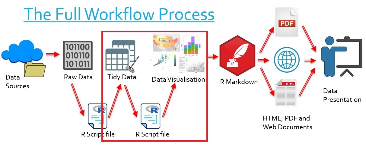
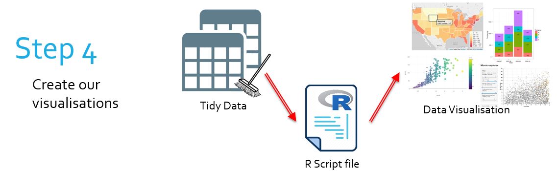
The Bigger Picture #

In this document we learn how to create interactive tables with DT. Simply put, we are learning how to transform tidy data into visually clear tables. In the overall context of the workflow, this falls into the category of transforming our data into data visualisation.

What is DT? #

LinkedIn Learning 6.1

library("tidyverse")
library("DT")

• An htmlwidget used to make interactive data tables from data frames and tibbles
• It is arguably the best R package for this specific purpose
• The package is bound to the DataTable library in JavaScript

Creating Interactive Tables #

LinkedIn Learning 6.2

Let’s say we have a dataset, such as the set below from the ACORN-SAT dataset. Note that we are deliberately using a large dataset (this one contains around 6000 observations)

load("tidy_ACORN-SAT_data/station_data.rdata")
head(station_data, 8)

##   Number year average.temp  Station.name Latitude Longitude Elevation Start
## 1   2012 1910         26.4   Halls Creek   -18.23    127.66       422  1910
## 2   3003 1910         27.3        Broome   -17.95    122.24         7  1910
## 3   6011 1910         21.5     Carnarvon   -24.89    113.67         4  1910
## 4   7045 1910         21.8   Meekatharra   -26.61    118.54       517  1926
## 5   9021 1910         18.0 Perth Airport   -31.93    115.98        15  1910
## 6   9518 1910         16.3  Cape Leeuwin   -34.37    115.14        13  1910
## 7   9789 1910         16.7     Esperance   -33.83    121.89        25  1910
## 8  10917 1910         15.0     Wandering   -32.67    116.67       275  1910

With DT, we can instantly make this an interactive table by using the pipeline (%>%) operator and piping our data into the datatable() function.

station_data %>%
  datatable()

We immediately have an interactive table. The remainder of this tutorial will address how to tweak the table we have. Currently here are some of the things we can do:

• View our data in an aesthetic table
• Show 10, 25, 50 or 100 observations at a given time using the drop-down menu
• View the another page of observations with the page feature below the table
• Click on the arrows next to the column names to order our observations in ascending or descending order by that variable name
• Search with the search bar for the occurence of a string in any column of an observation
  • Try typing “Tarcoola”
  • Now try typing “25.” What do you notice?

Additional Options #

We notice that the first ‘column’ is just a number representing which observation of the table we are looking at. This is generally of no purpose to us, so we can remove it using the rownames argument of datatable(). We set it to FALSE.

station_data %>%
  datatable(rownames = FALSE)

We also notice some of our column names are not very aesthetic. We can make them more so by:

• Using the gsub() and stringr::str_to_title() functions to create a list of nicer names
• Using the colnames argument of datatable() to change these names

The following command replaces all dots (.s) with spaces, then capitalises the first letter of each word, and stores the new set of names in the column_title variable.

column_titles <- gsub("[.]", " ", colnames(station_data)) %>%
  stringr::str_to_title()

column_titles

## [1] "Number"       "Year"         "Average Temp" "Station Name" "Latitude"    
## [6] "Longitude"    "Elevation"    "Start"

We now use these as the new column names with colnames:

station_data %>%
  datatable(rownames = FALSE,
            colnames = column_titles)

We can already search for a given term in our data, but if we want to search for a term in a single column, we can add individual column filters using the filter argument.

• This argument takes a list of sub-arguments as its value
• We set the position sub-argument to “top” or “bottom” to add our filter

station_data %>%
  datatable(rownames = FALSE,
            colnames = column_titles,
            filter = list(position = "top"))

If we wish to display a number of observations which is not 10, 25, 50 or 100, we can use the options argument,

• This argument takes a list of sub-arguments as its value
• We set the pageLength sub-argument to the number of observations we wish to display

station_data %>%
  datatable(rownames = FALSE,
            colnames = column_titles,
            options = list(pageLength = 7))

Now say we wish to modify the search bar so that it doesn’t say “Search:” but instead “Keyword look-up:”

• We still use the options argument of datatable()
• We use the sub-argument language of options, which itself takes a list as its argument
• We use the sub-sub-argument sSearch to rename the search bar

station_data %>%
  datatable(rownames = FALSE,
            colnames = column_titles,
            options = list(pageLength = 7,
                           language = list(sSearch = "Keyword look-up:")))

Formatting Values in Tables #

LinkedIn Learning 6.3

Sometimes we will wish to display data in specific formats, such as dollars ($), a percentage (%) or otherwise. We have specific functions in DT for each of these.

sample_price %>%
  datatable()

If we wish to format a column as a currency, we pipe our table into formatCurrency():

• The first argument is the column to format (as a string!!!)
• We then use the currency argument to select the currency we want (as a character)

sample_price %>%
  datatable() %>%
  formatCurrency("Amount_Spent",
                 currency = "$")

If we were dealing in another currency, such as the Japanese Yen, we can specify an alternate currency:

sample_price %>%
  datatable() %>%
  formatCurrency("Amount_Spent",
                 currency = "¥")

If we wish to change the decimal places displayed, we use the additional argument digits:

sample_price %>%
  datatable() %>%
  formatCurrency("Amount_Spent",
                 currency = "$") %>%
  formatCurrency("Budget",
                 currency = "$",
                 digits = 0)

Let’s say we now want to display the percentage of our budget we have spent.

sample_price <- sample_price %>%
  mutate(Portion_Spent = Amount_Spent / Budget)
sample_price

## # A tibble: 6 x 4
##   Date       Budget Amount_Spent Portion_Spent
##   <chr>       <dbl>        <dbl>         <dbl>
## 1 21-06-2019     50         49.2         0.984
## 2 22-06-2019     50         47.2         0.944
## 3 23-06-2019     50         41.8         0.836
## 4 24-06-2019     50         52.0         1.04 
## 5 25-06-2019     50         52.9         1.06 
## 6 26-06-2019     50         37.8         0.755

We use the formatPercentage() function, specifying:

• The column to format as the first argument
• The number of decimal places we require as the digits argument

sample_price %>%
  datatable() %>%
  formatCurrency("Amount_Spent",
                 currency = "$") %>%
  formatCurrency("Budget",
                 currency = "$",
                 digits = 0) %>%
  formatPercentage("Portion_Spent",
                 digits = 2)

Lastly, if we wish to format dates, we use the formatDate() function:

• We specify the column to format as the first argument
• We specify the method by which to format in the method column
  • We generally assign “toDateString,” but a full list of methods can be found here

sample_price %>%
  datatable() %>%
  formatCurrency("Amount_Spent",
                 currency = "$") %>%
  formatCurrency("Budget",
                 currency = "$",
                 digits = 0) %>%
  formatPercentage("Portion_Spent",
                 digits = 2) %>%
  formatDate("Date",
             method = "toDateString")

Here the date formating failed. The reason for this is that the “Date” column contains strings of D-M-Y formatted dates. The formatDate() function requires entries of class ‘date,’ not strings. We can fix this using the lubridate package.

• We mutate our Date column
• We use the dmy() function of lubridate because our dates are in D-M-Y format
• The entries are reclassified as dates

class(sample_price$Date)

## [1] "character"

library("lubridate")
sample_price <- sample_price %>%
  mutate(Date = dmy(Date))

class(sample_price$Date)

## [1] "Date"

sample_price %>%
  datatable() %>%
  formatCurrency("Amount_Spent",
                 currency = "$") %>%
  formatCurrency("Budget",
                 currency = "$",
                 digits = 0) %>%
  formatPercentage("Portion_Spent",
                 digits = 2) %>%
  formatDate("Date",
             method = "toDateString")

Options for Responsive Tables #

LinkedIn Learning 6.4

If we have tables with lots of columns, we have options to truncate these.

(Sample data provided by Climate Change in Australia)

fire_data %>%
  datatable(rownames = FALSE,
            options = list(pageLength = 5))

The simplest method is using the argument extensions of datatable().

• We can set this to “Responsive” to truncate columns
• These can then be viewed for individual data points

fire_data %>%
  datatable(rownames = FALSE,
            extensions = "Responsive",
            options = list(pageLength = 5))

We now have a + button that displays columns which can’t fit on our screen. There is, however, an even more responsive solution which allows the reader to select and deselect columns for viewing as they like. This requires some setup:

• We set the extensions argument to a vector containing “Responsive” and “Buttons” (ie `c(“Responsive,” “Buttons”))
• We add the sub-argument buttons to the options argument of datatable()
• This takes the value of I("colvis") since we want the column-visability button
  • Note: the reason we wrap this in the I() function is technical and relates to the formatting of DT
• We add the sub-argument dom to the options argument of datatable()
• This takes the value of “Bf” for our purposes
  • More on dom below

fire_data %>%
  datatable(rownames = FALSE,
            extensions = c("Responsive", "Buttons"),
            options = list(pageLength = 5,
                           buttons = I("colvis"),
                           dom = "Bf"))

We now have a “Column visibility” button we can use to toggle columns as displayed and hidden.

More on the dom Argument #

This argument controls much about what we see in our tables. The argument is always a string, but, unlike many arguments we have seen in R, it is the individual letters of the string that are important.

In the above example, “Bf” means we desire Buttons and filter to be enabled, in that order. There are actually many letters we can use to enhance or change our table (several of which are described here). We may be interested in:

(*) Of course the table is always enabled, but this option is important in controlling order. For example, if we want the filter to be below the table, we use dom = "tf":

station_data %>%
  datatable(rownames = FALSE,
            options = list(pageLength = 5,
                           dom = "tf"))

As another example, consider the argument “Bpiltf,” structuring the widget, from top to bottom, as buttons, page-navigation, summary info, length changing, the table, and the filter below:

station_data %>%
  datatable(rownames = FALSE,
            extensions = c("Responsive", "Buttons"),
            options = list(pageLength = 5,
                           buttons = I("colvis"),
                           dom = "Bpiltf"))

Lastly, as a fun example, consider that we are not limited to just one of each letter:

station_data %>%
  datatable(rownames = FALSE,
            options = list(pageLength = 5,
                           dom = "ppfptpf"))

Maybe this would not be such a good idea in practice!

Allowing Users to Download Table Data #

LinkedIn Learning 6.5

We can add a button which allows users to download the data as it appears in our table.

• Users may download the content straight from (for example) your HTML webpage
• Users also may filter or remove columns and download the modified table

To do this is very similar to how we added the “colvis” buttons:

• Include the extensions argument of datatable()
• Set this to c("Responsive", "Buttons")
• Include the options argument of datatable()
• Set this to a list, containing the sub-argument buttons
• Set the value of this sub-argument to a vector of “excel” and “csv”

station_data %>%
  datatable(rownames = FALSE,
            extensions = c("Responsive", "Buttons"),
            options = list(pageLength = 5,
                           buttons = c("colvis", "excel", "csv"),
                           dom = "Bf"))